Go fast by letting go of the past (derivatives in your numerical optimization).

Synthetic controls are great. Instead of worrying about having no clean control group in your data to estimate a treatment effect, just create one! No wonder they’ve been called the biggest innovation in policy evaluation in the last decade. It’s what MacGuyver would do if he did causal inference.

Abadie (2021) has the go-to recipe for creating synthetic controls.¹ Basically it’s a weighted sum of all the non-treated groups. The main rub is that you derive the optimal weights through interpolation rather than extrapolation. Instead of running a regression, you set up a quadratic program with two linear constraints and solve it with sequential least squares programming.

Interpolation keeps your synthetic control from over-fitting in the pre-treatment and thus ensures valid inferences post-treatment. But a potential downside to this approach is that it can be slow, especially if you have a large “donor pool” of units who could plausibly contribute to the synthetic control.

The good news is that a few tweaks to your code can speed things up considerably. And by tweaks I mean just choosing a different optimization method and adding a regularization to the objective function. This speed-up may be useful if you’re spinning up lots of synthetic controls (or synthetic controls from large data) on the fly.

I stumbled onto this finding the other day while replicating the famous Cigarette Tax paper by Abadie, Diamond and Hainmueller (2010). Before diving into the optimization stuff, let’s review the paper.

Sin taxes

Consider a tax on cigarettes. Will it curb smoking? The price of smokes goes up, so demand should go down. On the other hand, the tax could have no effect because cigarettes are addictive, meaning demand is inelastic and thus brittle to price changes.

California levied such a cigarette tax back in 1988. Abadie and friends looked at whether the tax caused a decrease in packs purchased. In causalspeak, the tax was was a “natural experiment” to which California smokers were “treated”. To see if smokers puffed less because of the tax, you just need to compare them to smokers in another state exposed to no tax.

The problem is that no state meets the requirement of resembling California in every regard expect this cigarette tax. However, many states, while not identical to California, are quite similar. So, if you could just take a dash of Oregon, and a mix it with a dash of Nevada, and a host of other states, you could create a fake California that is just like the real California, only without the tax. The causal effect of the tax is then simply the difference between the real and fake California.

TLDR, the tax did indeed cause a decrease in cigarette consumption, as seen by the gap in the lines after 1988:

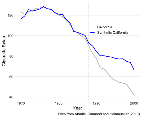
But how exactly do you make a fake California? The authors show how you can use numerical optimization to construct such “synthetic controls” and solve causal mysteries when randomized trials are impossible. What I found is that there are some simple ways you can speed up this optimization.

Cooking up a California

The first problem in creating a synthetic control is the fundamental problem of causal inference. It’s simply the fact that you can’t take the pill and placebo at the same time.

Let $Y_t^{I}$ be packs bought by smokers in California in year $t$ with intervention $I$ (the cigarette tax). Let $Y_t^N$ be packs bought by smokers in the control group – that is, California without the intervention. The treatment effect of the tax in $t$ is simply the difference between these numbers. The problem is you observe $Y_t^{I}$ but not $Y_t^{N}$. So, you need an estimate of $Y_t^{N}$.

The synthetic control estimates $Y_t^{N}$ from other states. In total we have $J+1$ states indexed by $j$. If $j=1$ is California, the treated state, then $j = {2, …, J+1}$ are the other states. Which brings us to the second problem in creating a synthetic control: finding the right mixture of these states to produce a $Y_t^{N}$ that resembles California.

So let’s add $j$’s to the mix. If each dash or weight for state $j$ is $w_j$ then the synthetic control is

and the problem is to find a vector of weights $\mathbf{w}$ that minimizes the difference between pre-treatment California ($\mathbf{X}_{j=1}$ or $\mathbf{X}_{1}$) and pre-treatment everywhere else ($\mathbf{X}_{j\neq1}$ or $\mathbf{X}_{0})$. If we let the difference be modeled as the L2 norm, where

then we have an objective function

subject to two constraints that ensure the solution $\mathbf{w}^*$ is a convex combination:

1. Each weight is between 0 and 1 ($0 \leq w_j \leq 1$),
2. The sum of the weights is 1 ($\sum_{j=2}^{J+1} w_j = 1$).

These constraints turn the problem into one of interpolation rather than extrapolation. Abadie gives a nice explanation of the tradeoff in an online talk, and so does Matheus Facure Alves in his excellent (and hilarious) book. The punchline is that extrapolation, say with linear regression, will produce a synthetic control that overfits pre-treatment California, which reduces your ability to make post-treatment comparisons.²

Anyways, how should we numerically solve this constrained optimization problem? I’ll focus on the heavyweight champion and a featherweight contender.

Choose your optimizer

The heavyweight champ: SLSQP

Since the objective function is twice differentiable, and since we have two inequality constraints, sequential (least-squares) quadratic programming (SLSQP) is an obvious choice. Mostly because it will guarantee a solution within the constraints.

The canonical algorithm is given by Kraft (1988) and implemented in the open-source non-linear optimization library NLOpt. You can access the SLSQP routine in NLOpt in R withnloptr::slsqp (source) and in Python with scipy.optimize.fmin_slsqp (source). ³ They produce the same results, so the choice of programming language is not a big deal.

Here it is in R. First the L2 norm:

1
2
3
4
l2norm = function(w){
  wstar = sqrt(mean((X1 - X0 %*% w)^2)) 
  return(wstar)
} 

Now the optimization. nloptr::slsqp lets you directly the lower and upper bound constraint on each weight via lower and upper, and you can set the second inequality constraint – all weights sum to one – with heq argument. If you have $N$ weights, the idea is that you optimize $N-1$ weights, and the last weight has to equal the sum of those weights minus one.

Finally, you set starting values with x0. You can be fancy and seed the optimizer with the regression coefficients $(\mathbf{X_0}^T \mathbf{X_0})^{-1} \mathbf{X_0}^T\mathbf{X_1}$ . But you can also just set the starting values equal to zero or one or $1/N$. If the solution is stable then the starting values should not matter too much.

1
2
3
4
5
6
7
8
9
10
# get N weights to optimize, one per state in the donor pool
N = ncol(X0)
# slsqp returns a list
m = nloptr::slsqp(fn = l2norm,
                  x0 = rep(1/N, N),
                  lower = rep(0, N),
                  upper = rep(1, N),
                  heq = function(x) sum(x) - 1)
# the optimal weights
wstar = m$par                                          

The featherweight contender: L-BFGS-B

Numerical optimization is iterative (“if at first you don’t succeed…”), and SLSQP uses the Broyden–Fletcher–Goldfarb–Shanno algorithm (BFGS) to numerically compute derivatives at each iteration. The problem is that BFGS stores all the gradients (first derivatives) and Hessians (second derivatives) from each sweep. Holding onto the past is a good thing, here at least, because it ensures a better approximation of the objective function’s curvature. But the price is speed. Iterate long enough and you end up using a good chunk of memory.

Limited-memory BFGS is BFGS but with less baggage. Over time it drops past derivative approximations to free-up memory. So it’s faster, at the price of accuracy. But if your optimization problem has a stable solution, then my thinking was that this accuracy cost should not bite too much. More good news, L-BFGS-B is an extension that lets you set box constraints like $0 \leq w_j \leq 1$. And you easily implement it in R with the built-in optimizer optim().

The only twist is that you cannot directly set the inequality constraint $\sum_{j=2}^{J+1} w_j = 1$. This one is crucial because it ensures the solution interpolates rather than extrapolates.

You can get around this by tweaking the objective function with regularization. By that I mean you just add a large term to the sum of the $N-1$ weights to kick any weight greater than one out of the solution:

1
2
3
4
5
l2norm = function(w){
  wstar = sqrt(mean((y - X %*% w)^2))
  wstar_penalized = abs(1e6 * (sum(wstar) - 1))
  return(wstar_penalized)
}

and then optimize:

1
2
3
4
5
6
7
8
# optim also returns a list
m = optim(fn = l2norm, 
         par =  rep(1/N, N), # starting values
         method = 'L-BFGS-B',
         lower = rep(0, N), 
         upper = rep(1, N))
# the optimal weights
m$par          

Results

The authors do inference with a permutation test. Pretend each state could have received the cigarette tax (the treatment), derive it’s synthetic control, and calculate the average treatment effect for each year. This approach makes it easy to estimate the distribution of treatment effects regardless of sample size.

I replicated the permutation test using both optimization approaches. In the plots below California is in blue and all the other states are in gray. Each line shows the difference between observed cigarette sales for state $j$ and sales for its synthetic control. The dotted line marks the treatment. You can see that sales dropped significantly in California because of the tax. More relevant to this note, you can also that the two optimization routines produce nearly identical results:

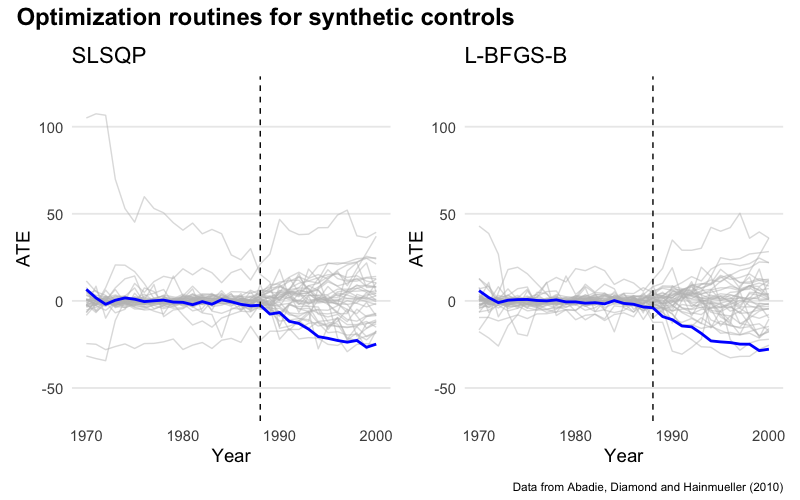
Permutation tests are computationally intensive. Here we’re solving 39 quadratic programs. Imagine if the donor pool were even bigger!

So, I ran a horse race, timing 100 sweeps of each optimization routine with the microbenchmark package. Here is the distribution of timings:

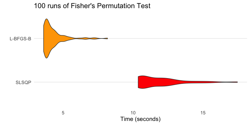
L-BFGS-B can produce the same results up 5x faster. Not bad!

Caveats

This was a quick-and-dirty experiment, so I don’t know all the fail points. One obvious issue is that L-BFGS-B can be tricked into forcing all weights to sum to one. But that does not mean the solution will sum exactly to one (in my experiments the solutions were usually between 0.9 and 1.0). SLSQP, by contrast, guarantees this constraint. As a result you may find slight differences in the optimal weights. Depending on the research question at hand this may or may not be an issue.

Perhaps a more pressing issue is uniqueness. If there are multiple feasible solutions, it’s plausible that different optimization approaches will yield quite different results. Abadie and L’Hour 2021) confront this problem head on by injecting a regularization directly into the quadratic program, which you could presumably run either with SLSQP or L-BFGS-B.

Code

The code to replicate this note is on GitHub.