Derivatives in PyTorch
January 2023
Exploring the autograd machinery of PyTorch with a linear model.
Took me time to see that lots of stats/machine learning/data science/whatever is really just about optimization. You have some data, you define a function to describe that data (like a likelihood function or a loss function), then you optimize that function using calculus. People have done this in some shape or form since the 1700s. Only nowadays we have tools like PyTorch to do the calculus for us (alongside other crucial science tools, like instant coffee and Spotify).
PyTorch is a Python interface for Torch, an open-source library for deep learning – neural networks with more than one layer.1 You need derivatives to optimize a function, and PyTorch has machinery called autograd to get those derivates.
The help pages discuss it better than I could. But I wanted to get a feel for how it worked, so here is a demo with a simple linear model. I’ll run the model with NumPy, then with PyTorch, and then show how both approaches yield the exact same results.
Optimization with gradient descent
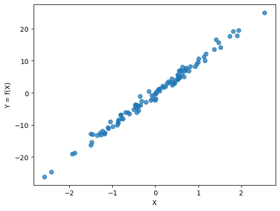
Say you have data generated by the linear model
\[y_i = \beta_0 + \beta_1 x_i + \varepsilon_i\]where $x_i$ and $y_i$ are data, $\beta_0$ and $\beta_1$ are parameters, and $\varepsilon_i \sim N(0, \sigma^2)$ is white noise. Say $\beta_0 = 0$ and $\beta_1 = 10$. Then:
1
2
3
4
5
6
7
import numpy as np

N = 100
X = np.random.normal(0,1,N)
e = np.random.normal(0,1,N)
b_true = 10.
Y = 0 + b_true*X + e
You could just use the closed-form solution to estimate $\beta_0$ and $\beta_1$ ($\mathbf{\beta} = (\mathbf{X}’\mathbf{X})^{-1} \mathbf{X}’ \mathbf{Y}$) but PyTorch uses gradient descent, so I’ll use that.
In the workhorse numerical optimization technique that is gradient descent, we descend to the solution along the gradient. That is, we define a function, ask how it changes at different values of the parameters, and go where the gradient – the vector of first derivatives – tells us to go to minimize the loss.
Let our loss function be the mean squared error between observed and predicted values:
\[\begin{aligned} L(\beta) &= \frac{1}{2N} \sum_{i=1}^N(f_{\hat{\beta}}(x_i) - y_i)^2 \\ &= \frac{1}{2N} \sum_{i=1}^N(\hat{\beta}x_i - y_i)^2 \end{aligned}\]In gradient descent we use the derivative of the loss function to evaluate how close we are to the solution:
\[\begin{aligned} L'(\beta) &= \frac{\partial L}{\partial \beta} \\ &= \frac{1}{N}\sum_{i=1}^N x_i(\beta x_i - y_i) \end{aligned}\]The goal is to find a value of $\beta$ through trial and error that satisfies the first-order condition of an optimization problem, $L’(\beta) = 0$.
So we define a Python function for the derivative:
1
2
def dL(beta, x, y):
    return np.mean(x * (x*beta - y))
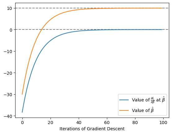
and then the idea is to start at some random value for $\beta$, calculate the derivative to see how the loss changes, and if the loss gets smaller, take a step in that direction, and do this many times until we satisfy, or at least approximate, $L’(\beta) = 0$. Formally:
\[\beta := \beta - \alpha \frac{\partial L}{\partial \beta}\]which means “update the estimated parameter according to gradient or derivative at that value and the step-size or learning rate $\alpha$”.
We have:
1
2
3
4
5
6
7
8
9
10
11
12
13
14
15
16
17
# initial guess for \beta_1
b = -30.

# step size / learning rate
step_size = 0.1

# empty list to store value of the gradient at each estimate of \beta_1
grad_list = []
# empty list to store each estimate of \beta_1
b_list = []

# run gradient descent 100 times
for i in range(100):
    b_list.append(b)
    dLdb = dL(beta = b, x = X, y= Y)
    grad_list.append(dLdb)
    b -= step_size * dLdb
After enough sweeps the first-order condition is satisfied, and the point estimate converges:
Gradient descent with PyTorch
To PyTorch-ify the code we first convert the NumPy arrays to tensors, and choose a starting value for $\beta_1$:
1
2
3
4
import torch
Xt = torch.tensor(X)
Yt = torch.tensor(Y)
b = torch.tensor(-30., requires_grad = True)
For this note we can just think of tensors as fancier NumPy arrays that have numerical differention properties. Setting requires_grad = True on a tensor means at some point we want its derivative – or in this case, the derivative of a loss function with respect to the tensor’s value.
Here is the main way in which the PyTorch version makes gradient descent easier. Unlike the NumPy version, where we used the derivative of the loss function, here we just need the loss function:
1
2
def L(beta, x, y):
    return 1/(2*N) * torch.sum((x*beta - y) ** 2)
and then in each sweep of our optimization we calculate the loss:
1
loss = L(beta = b, x = Xt, y = Yt)
and then evaluate the derivative of the loss function at a given value of b, $\frac{\partial L}{\partial \hat{\beta}}$, by simply calling
1
loss.backward()
The full program has a few extra bits, like clearing the gradient in each sweep (read why here):
1
2
3
4
5
6
7
8
9
10
11
12
# empty list to store value of the gradient at each estimate of \beta_1
grad_list2 = []
# empty list to store each estimate of \beta_1
b_list2 = []

for i in range(100):
    b_list2.append(np.array(b.data))
    loss = L(beta = b, x = Xt, y = Yt)
    loss.backward()
    grad_list2.append(np.array(b.grad.data))
    b.data -= step_size * b.grad.data
    b.grad.data.zero_() # clear the gradient
Comparing the two approaches
Both approaches yield a point estimate for $\beta_1$ of about 9.95, which is very close to the true value of 10. And both approaches arrive to that estimate the same way. Here are the first five values of the point estimate and the derivative of the loss function evaluated at the point estimate. You can see they are identical across the board:
| Iteration | Gradient (NumPy) | Gradient (PyTorch) | Estimate (NumPy) | Estimate (PyTorch) |
|---|---|---|---|---|
| 0 | -38.356 | -38.356 | -30.000 | -30.000 |
| 1 | -34.674 | -34.674 | -26.164 | -26.164 |
| 2 | -31.346 | -31.346 | -22.696 | -22.696 |
| 3 | -28.337 | -28.337 | -19.562 | -19.562 |
| 4 | -25.617 | -25.617 | -16.728 | -16.728 |
No surprise, really. Both programs do exactly the same thing. But the PyTorch approach is easier and more generalizable. You simply use the loss function rather than its derivative.
FullTorch
For the sake of completion let’s fully torch-ify the program.
First we’ll generate some data where $\beta_0 = 0$ and $\beta_1 = 10$ and ensure it’s nicely shaped:
1
2
3
4
5
6
7
8
N = 100
X = np.random.normal(0,1,N).reshape(-1,1)
e = np.random.normal(0,1,N).reshape(-1,1)
b_true = 10.
Y = 0 + b_true*X + e

Yt = torch.tensor(Y, dtype = torch.float32)
Xt = torch.tensor(X, dtype = torch.float32)
Then we define our model as a torch.nn.Module, a neural network model with a transformation and “forward pass” (basically the prediction):
1
2
3
4
5
6
7
8
class LinReg(torch.nn.Module):
    def __init__(self, inputSize, outputSize):
        super(LinReg, self).__init__()
        self.linear = torch.nn.Linear(inputSize, outputSize)

    def forward(self, x): # like predict() in R
        yhat = self.linear(x)
        return yhat
and then create a model object from the LinReg class, where inputSize and outputSize are 1 because we have a $n \times 1$ vector for $\mathbf{X}$ and $\mathbf{Y}$:
1
model = LinReg(inputSize = 1, outputSize = 1)
Next we define our loss function using PyTorch’s built-in mean-squared error loss, and then call built-in optimizer, stochastic gradient descent:
1
2
loss_function = torch.nn.MSELoss()
optimizer = torch.optim.SGD(model.parameters(), lr=0.1)
and away we go:
1
2
3
4
5
6
for i in range(100):
    optimizer.zero_grad()
    Yhat = model(Xt)
    loss = loss_function(Yhat, Yt)
    loss.backward()
    optimizer.step()
The program gives us good estimates, as expected:
1
2
3
4
5
6
7
for name, param in model.named_parameters():
    print(name, param)

linear.weight Parameter containing:
tensor([[9.9119]], requires_grad=True)
linear.bias Parameter containing:
tensor([-0.1741], requires_grad=True)
Code
The code to replicate this note – including a PyTorch program for multiple linear regression – is available on GitHub.
-
Recall that a neural network with one layer is just logistic regression. ↩