Modeling seasonality with sines and cosines.

Forgive the pun. Lately I’ve been thinking about Fourier series. Consider the additive time series model:

\[y(t) = g(t) + s(t) + \epsilon(t)\]

where $t$ is time, $g(t)$ is trend, $s(t)$ is seasonality, and $\epsilon(t)$ is randomness.

When building a forecast of $y(t)$ there are lots of ways to model $s(t)$. The simplest way is to use dummy variables and let the intercept of the regression line move up and down with the seasonal pattern. But those dummies eat up your degrees of freedom if there is complex seasonality (e.g., distinct patterns by day, month and year).

Fourier series are a nice alternative. Facebook uses them for their forecasting tool Prophet, and they’ve been around awhile now in the literature on dynamic linear models. The idea is that any complex, periodic function like $s(t)$ can be approximated as a sum of just a few sines and cosines. A bit like how General Additive Models approximate complex non-linear functions with a bunch of simple basis functions like polynomials or splines.

To see how this works let’s take a simple example from the signal processing literature.

The Fourier Transform

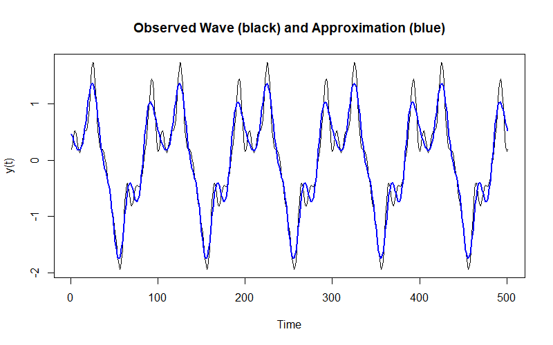
Say you observe this wave:

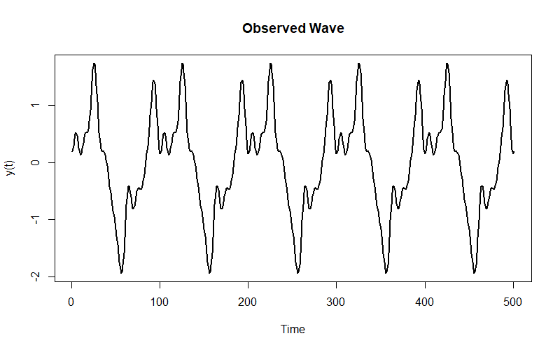
It’s actually the sum of these ten harmonics (that I made up) evaluated over a sequence of time values $t \in T$:

\[y_t = \sum_{k = 1}^{10} \frac{1}{k} \sin(2\pi k t + k^2)\]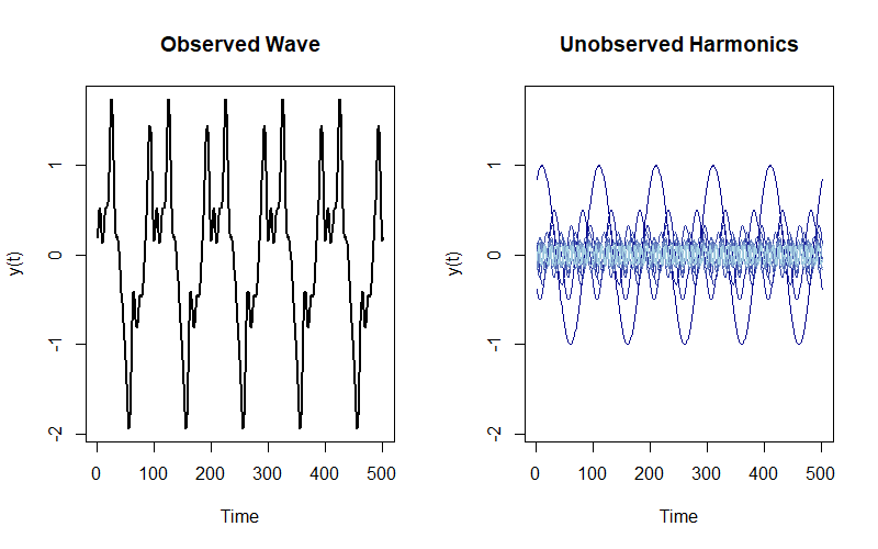

But you don’t observe these harmonics. How can you recover their attributes to approximate the wave you observe? Enter the Discrete Fourier Transform (DFT).

The DFT converts $y_t$ from time to frequency:

\[Y_k = \sum_{t=0}^{T-1}{y_t e^{-i2\pi kt/T}} = \sum_{t=0}^{T-1}{y_t[\cos(2\pi{kt/T}) -i\sin(2\pi{kt/T})]}\]

where $Y_k$ is the $k$-th Fourier Coefficient and $i$ is an imaginary number ($i = \sqrt{-1}$). That is, each coefficient is a complex exponential with a real and imaginary component containing the amplitudes of the underlying harmonics to the observed wave. (A complex exponential is just $e^{ix} = \cos(x) + i\sin(x)$, and recall that $\sin(x) = \cos(x + \frac{\pi}{2})$, i.e., a cosine is just a sine with a 90 degree phase shift.)

The Fast Fourier Transform carries out the DFT and returns those $k$ coefficients. For instance, the second coefficient $k=2$ is about $0.22-0.06i$, which means the amplitude of the corresponding cosine is 0.22 and the amplitude of the corresponding sine is -0.06.

For each $k$ coefficient we can construct these waves using the Inverse Fourier Transform and recover the original wave:

\[y_t = \frac{1}{T}\sum_{t=0}^{T-1}{Y_k e^{i2\pi kt/T}} = \frac{1}{T}\sum_{t=0}^{T-1}{Re(Y_k)\cos(2\pi{kt/T}) + Im(Y_k)\sin(2\pi{kt/T})]}\]

where $Re(Y_k)$ is the real component of $Y_k$ (0.22 in the example) and $Im(Y_k)$ is the imaginary component (-0.06).

There are $k = T$ coefficients. If you do the inverse transform using all all of them you recover the original wave:

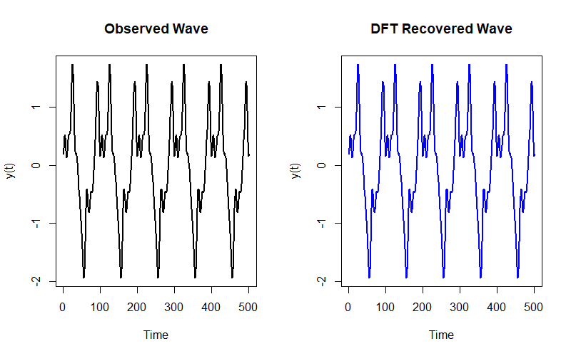
But what if we just want to approximate the wave? Notice how most of the $k$ coefficients are quite small:

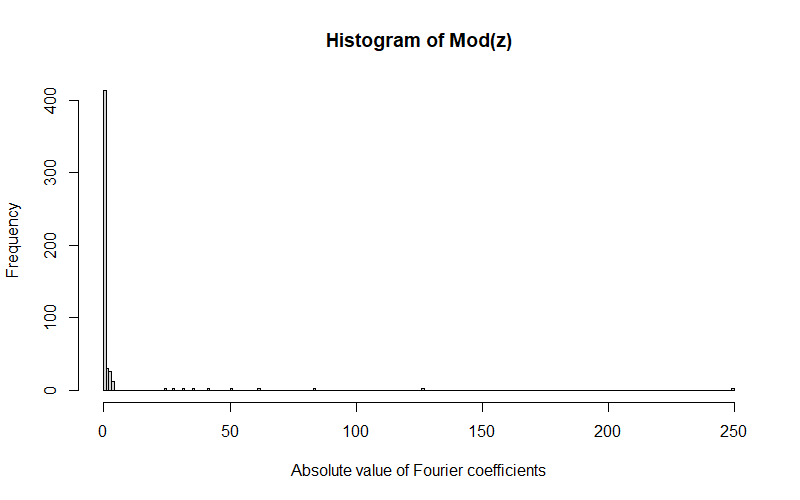
so we can ignore them and get a decent approximation with, say, the ten largest coefficients:

Dynamic harmonic regression

You don’t actually do a DFT when using Fourier series to model the seasonality component $s(t)$ in a time series model. But the basic idea is the same: approximate $s(t)$ with a bunch of sines and cosines. The main difference is that instead of a DFT you run a regression and pick how many sines and cosines to include in advance.

The goal is to estimate

\[s(t) = X(t)\mathbf{\beta}\]

where $X(t)$ is a $K \times N, k \in K$ matrix of sines and cosines. You’re modeling $s(t)$ as

\[s(t) \approx a_0+ \sum_{k = 1}^K {y_t[a_k\cos(2\pi{kt/T}) + b_k\sin(2\pi{kt/T})]}\]

which resembles the inverse DFT.

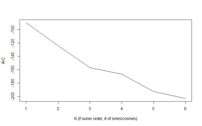
So how many sines and cosines should you throw into $X(t)$? You want to get a good approximation without overfitting. The standard approach is to minimize some information criterion like the AIC ($2k - 2L$, where $L$ is the likelihood).

Consider wine data sales from the forecast package by Rob Hyndman (check out his book):

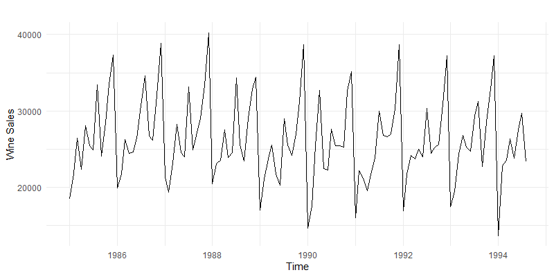
As we increase the number of sines and cosines in $X(t)$ we get a better fit:

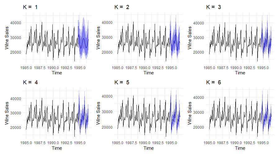
and we minimize the AIC:

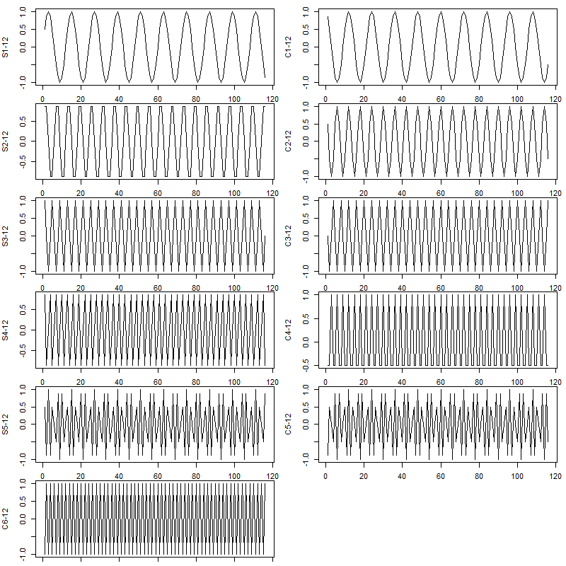
and under the hood it’s just a Fourier series, a bunch of sines and cosines added up to approximate $s(t)$:

And to think, Joseph Fourier figured all this out almost 200 years ago, without the internet.

Code

The code to reproduce the figures is on GitHub.