But at what price?

Simple interactions can produce complex phenomena. Take for example a starling murmuration. There is no maestro leading the flock who says, “okay everyone, just like we rehearsed”. Each starling just flies. And yet when you add them all up they become a single shapeshifting entity, a whole much greater than the sum of its parts.¹

Computer simulations known as agent-based models (ABM) are a standard tool for studying complexity and emergence. And with Python – one of the most popular languages – you can quickly prototype a proof-of-concept. But speeding up the code can be tough. This matters because the discovery payoffs to speed-ups can be huge. Faster code lets you run more experiments and dive deeper and longer and into the world you are modeling.

Python is slow relative to other languages (e.g., C/C++, Fortran, Java) by design: the price of fast development (writing code) is slow execution (running code). But another reason is the general nature of an ABM. Its speed is a function of how many times the model is run and how many agents are involved, regardless of the programming language.

Your garden variety ABM has two components: a loop over $M$ sweeps or runs, and inside each sweep, a loop over $N$ agents (starlings, or people, or whatever). Something like this:

1
2
3
for each run in M:
    for each agent in N:
        interact

The computational complexity of that pseudocode – ignoring what agents actually do in those interactions – is $O(M \times N)$. Increase the number of runs, or the number of agents, or both, and the model will take longer to run. I was in this position with a recent project. To speed-up progress I had to speed-up the code.

Fortunately there are ways to avoid getting hammered by this $M$-and-$N$ tradeoff in Python. NumPy can run lots of agents ($N$) and Numba can run lots of, well, runs ($M$). Put them together and you have a solid one-two punch.²

To test it I coded up a simple model five different ways and ran a horse race. (All the code is online.) It was a nice little exercise: given a baseline model written in pure Python, how can you speed it up, and more importantly, what are the net benefits?

In terms of runtime the NumPy + Numba implementation is the clear winner. But it came at a steep price, mainly because of NumPy. I had to completely re-think how to code the model, and the end product was hard to read. The speed tests show that there is no point paying the marginal development cost of NumPy unless your model has tons of agents. Numba on the other hand is pretty easy to deploy, so long as you’re willing to re-write just a few things with NumPy.

A simple model of income inequality

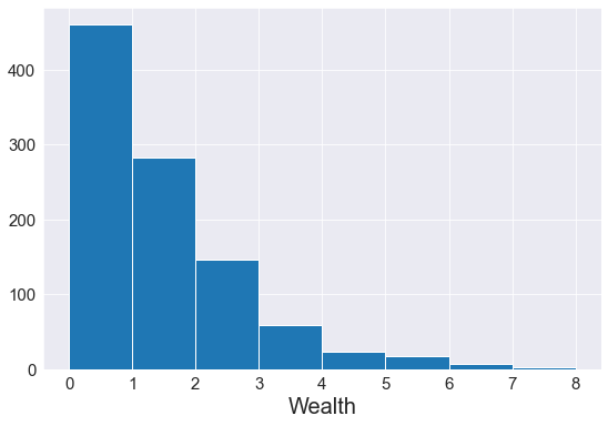
Picture a population of agents who start their lives with one dollar. In each sweep of the model they check their bank account. If they have funds they choose a different agent at random and give them a dollar. That’s it.³

What emerges over time is an income distribution with a few haves and many have-nots. It’s a simple world where a few agents get rich because they get lucky early on. Here is what you get with one hundred agents starting off with uniform wealth and then interacting for one hundred runs:

Implementing the model

There are many ways to code this model. The biggest choice is how to represent the agents.

Like their organic cousins, computer agents are data structures, only simpler. In a “native” or pure Python model an agent is a list with two elements, agent = [ID, wealth], that you can index (e.g., to access an agent’s wealth, the second element: agent[1]).

Alternatively you could code a model with object-orientation (OO): an agent is a bespoke object with attributes (identification, wealth) and methods (pick a neighbor at random and give them a dollar).

However, both lists and OO are slow for large $N$. You can speed up the model by using different data structures for the agents. This is where NumPy comes in.

NumPy

NumPy is the standard go-to for $N$ bottlenecks. First, Python lists are replaced with NumPy arrays, which use less memory. Second, and more importantly, Python loops are replaced with “vectorization” (basically, math on arrays of like sizes) and “broadcasting” (math on arrays of different sizes). Vectorization and broadcasting run loops in C rather than Python. That means NumPy will be a lot faster when manipulating, say, a population of agents, so long as they are stored in a NumPy array.

For instance, if I wanted to gift every agent in population $a$ one dollar, I could do this:

1
2
for agent in a: # an agent is [ID, wealth]
    agent[1] += 1 # agent[1] -> second element of agent's list is their wealth

where a is the agent population, a list-of-lists (e.g., [[1, 1], [2, 1]]). If instead a were a NumPy array I could just do:

1
a[:,1] += 1

which runs the same loop but in C.

Lots of Python can be swapped for NumPy. But it’s no free lunch. Where Python is easy to read, NumPy can be downright baffling. I’ll show this in a minute.

Switching to NumPy won’t necessarily reduce the complexity of the Python program – it will just speed it up by doing the heavy lifting (loops over $N$) in a faster language. But it won’t do much for $M$, since that loop is still written in native Python.

Numba

We can attack the $M$ bottleneck with Numba. Numba is like a performance-enhancing drug. It compiles Python code into machine code (LLVM, specifically) that runs at speeds close to C, C++ or Fortran. All this with minimal effort: take your program and just add a decorator on top of it. For instance, this model:

1
2
3
4
def abm(n_runs, n_agents):
    for run in range(n_runs):
        for agent in range(n_agents):
            # interact

can be “jitted” (made to compile just-in-time) by adding the cherry @numba.njit on top:

1
2
3
4
5
@numba.njit # same as "@jit(nopython=True)"
def abm(n_runs, n_agents):
    for run in range(n_runs):
        for agent in range(n_agents):
            # interact

The decorator @numba.njit means “compile the function without Python” (the “n” is for “no Python”) and it’s the number-one (sorry, “numba-one”) performance tip.

The only caveat is that Numba prefers certain data types, namely NumPy arrays over native lists. And it only supports certain NumPy functions (though the list is growing).⁴

The horse race

I coded up five versions of the income-dynamics model above (here is the Jupyter Notebook). The model is so simple that any major speed differences will be driven by runs $M$ and agents $N$ (and not the fact that I wrote the code instead of somebody else).

1. Native: object-orientation (OO)
2. Native: lists (non-OO)
3. NumPy
4. Numba + NumPy
5. Numba + Mixed

Numpy for $N$

The first three implementations vary how agents are represented:

1. as bespoke objects (i.e., class agent(object));
2. as $1 \times 2$ lists ([id, wealth]); or
3. as NumPy arrays.

The NumPy implementation eliminates Python loops with a few backflips. Each agent is a $1 \times 4$ array (so the whole population is $N \times 4$). The first element stores the agent’s ID and the second element stores the ID of a randomly chosen neighbor in a given round and to whom they give a dollar (funds permitting). The third element stores the number of times the agent in question got their number called (and thus the number of dollars they “earn” that round, subject to the rules of the game). The last and fourth element stores the agent’s total wealth.

This approach lets you work over the agent population all at once rather than one agent at a time. But it also underscores the speed-legibility tradeoff, because NumPy code that replaces native loops can take long to write and be hard to read.

In the native, non-OO version the loop over agents looks like this:

1
2
3
4
5
6
7
# "a" is the list-of-list agent population; an agent is [id, wealth]
for agent in a: # for each agent, you
    if agent[1] > 0: # check if you have funds, and if so
        other_agent = random.choice(a) # pick another agent at random
        if agent[0] != other_agent[0]: # and if they have have a different id than you
            other_agent[1] += 1 # give them a dollar...
            agent[1] -= 1 # ...from your bank account

which is pretty easy to follow. By contrast, here is my NumPy version:

1
2
3
4
5
# "a" is the numpy array agent population
a[:,1] = np.random.choice(a[:,0],n_agents, replace=True)
a[:,2] = np.bincount(a[(a[:,3]>0) & (a[:,0] != a[:,1])][:,1], minlength=n_agents)
a[:,3][(a[:,3] > 0) & (a[:,0] != a[:,1])] -= 1
a[:,3] += a[:,2]

Both implementations do the same thing (the Jupyter notebook shows the output all the implementations). But the NumPy version took longer to write and it’s harder to read, bearing no resemblance to its native counterpart. A very bad deal for models with small numbers of agents, as the speed tests demonstrate.

Numba for $M$

Then the Numba implementations. Version (4) just sticks a decorator on top of (3), while version (5) is a “mixed” implementation that tries to strike a balance between speed and legibility by using both NumPy and native loops:

1
2
3
4
5
6
for agent in a: # "a" is now a numpy array
    if agent[1] > 0:
        other_agent = a[np.random.choice(np.arange(n_agents)),:] # pick a random agent = pick a random row in the array
        if agent[0] != other_agent[0]:
            other_agent[1] += 1
            agent[1] -= 1

Unfortunately I ran out of time to try an implementation that combines OO with Numba. That would have been nice because OO programming is very intuitive for ABMs. You can jit an entire class, or you can jit a method function within a class, but both approaches seem to be more time consuming than just sticking the Numba decorator on top of a working non-OO version.

Results

I timed each model by running it five times (ten loops each time) and taking the average. First I ran a test on $M$, the number of runs, holding constant the number of agents ($N=100$).

Sure enough, the biggest speed gains for large $M$ come from Numba:

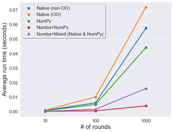
By contrast, the speed gains from NumPy are slim. No surprise, since NumPy works on $N$. So if you’re running a model with a small number of agents and lots of rounds, it makes no sense to NumPy-ify the code.

NumPy does make sense if you’re running lots of agents. The tests below vary $N$ and hold constant the number of runs ($M=100$):

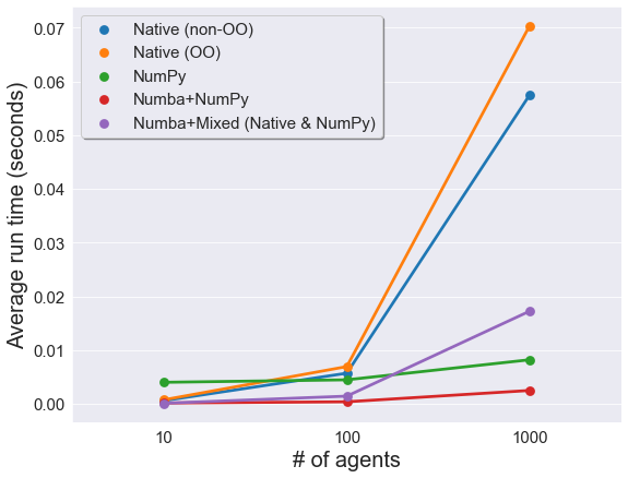
Not only is NumPy fast for large $N$, it’s faster than the “mixed” Numba implementation. No surprise, really. NumPy is just very good at what it does. Even so, after having to code the NumPy version I rooted against it.

A song of $M$ and $N$

Long story short: only use NumPy if your ABM has a ton of agents ($N$). Then use Numba to quickly run lots of rounds ($M$). Do neither until you know the model works with a few agents and a few rounds. Premature optimization is the root of all evil, and all that.

Of course, you don’t even need a computer to run a simulation. Schelling ran his segregation model on a chessboard back in 1978 – 13 years before Python was invented, 28 years before NumPy, and 34 years before Numba.⁵ A friend of mine joked that the ideal ABM would involve real people interacting with each other in some physical space. Sounds like a gas. Maybe Mr. Burns will fund it.

Code

The code to replicate this note is on GitHub.