Clustered standard errors by hand
May 2022
Average treatment effects are cool and all, but what about the standard errors?
I spent way too long in grad school thinking about clustered standard errors. What is the big deal? How do you do them? What am I doing with my life? Just grad school things.
Anyway, I worked out an example of how to cluster standard errors by hand for a lecture in one of my graduate courses, and it helped me better appreciate the general problem of non-constant variance in the linear model.
This stuff is especially important when estimating average treatment effects in experiments. So here is a demo using one of my favorite experimental papers about the evolutionary origins of loss aversion.
But first, the linear model.
Variance is probably never constant
In a linear model we assume that data are generated by
\[y = \mathbf{X}\beta + \epsilon\]where $y$ is a $n \times 1$ response vector, $\mathbf{X}$ is a $n \times k$ data matrix, $\beta$ is a $k \times 1$ coefficient vector, and $\epsilon$ is a $n \times 1$ error vector that captures variance in $y$ not captured by $\mathbf{X}$.
Ordinary Least Squares (OLS) is the standard way to estimate the parameters of our model $\beta$, and one of its assumptions is that the error is normally distributed and constant across observations: $\epsilon \sim N(0,\sigma^2)$.
What does it mean to assume constant variance? It means our model believes $\epsilon$ is the same around each data point.
This assumption is usually wrong. But how we are wrong? Assuming constant variance does not impact our estimates of $\beta$, it impacts our inference about $\beta$.
Heteroskedasticity
Heteroskedasticity is a common form of non-constant variance. Suppose we observe 100 different individuals with 100 different incomes:
1
df = data.frame(x = 1:100)
and let’s suppose their consumption $y$ (including debt – it’s a loose model here) is a linear function of their income $x$ and some unobservables:
\[y_i = 2x_i + \epsilon_i\]where $\epsilon_i = \epsilon \sim N(0, \sigma^2)$. Let’s assume $\sigma^2 = 400$ (or equivalently, $\sigma = 20$):
1
2
3
set.seed(1234)
df = df %>%
  mutate(y = 2*x + rnorm(n = 100, mean = 0, sd = 20))
Plotting income against consumption shows that the spread around the regression line is constant:
1
2
3
4
5
df %>%
  ggplot(aes(x = x, y = y)) +
  geom_point() +
  geom_smooth(method = 'lm', formula = 'y ~ x') +
  labs(x = "Income", y = "Consumption")
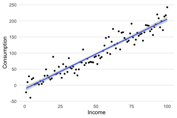
But do we really believe that the variance in consumption is constant with income? We should expect the opposite. When your income goes up, you can consume a larger basket of goods. Now that you finished grad school you eat lobster five days a week, and ramen the other days, just to keep it real.
Let’s add a new consumption variable that relaxes the assumption of constant variance. Instead we’ll assume that $\epsilon$ is a function of income, $\epsilon_i \sim N(0, x_i^{1.7})$:
1
2
3
set.seed(1234)
df = df %>%
  mutate(y2 = 2*x + rnorm(n = 100, mean = 0, sd = x^1.7))
Now you can see how the variance in consumption increases with income:
1
2
3
4
5
df %>%
  ggplot(aes(x = x, y = y2)) +
  geom_point() +
  geom_smooth(method = 'lm', formula = 'y ~ x') +
  labs(x = "Income", y = "Consumption")
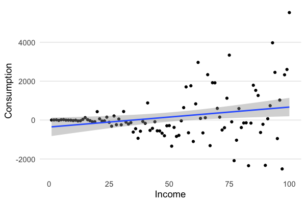
So what? When we estimate the parameters:
1
2
library(fixest) # https://lrberge.github.io/fixest/
hksd_model = fixest::feols(y2 ~ x + 0, data = df)
Our estimate of $\beta$ is not affected by whether we account for non-constant variance, but our inference is.
Here we don’t adjust for non-constant variance:
1
summary(hksd_model)
1
2
3
4
5
6
7
8
OLS estimation, Dep. Var.: y2
Observations: 100
Standard-errors: IID
  Estimate Std. Error t value Pr(>|t|)
x  4.91329    2.07685 2.36574 0.019942 *
---
Signif. codes:  0 '***' 0.001 '**' 0.01 '*' 0.05 '.' 0.1 ' ' 1
RMSE: 1,202.0   Adj. R2: 0.027656
and here we do (using the usual Huber-White adjustment):
1
summary(hksd_model, se = "hetero")
1
2
3
4
5
6
7
8
OLS estimation, Dep. Var.: y2
Observations: 100
Standard-errors: Heteroskedasticity-robust
  Estimate Std. Error t value Pr(>|t|)
x  4.91329    2.96231  1.6586  0.10036
---
Signif. codes:  0 '***' 0.001 '**' 0.01 '*' 0.05 '.' 0.1 ' ' 1
RMSE: 1,202.0   Adj. R2: 0.027656
Notice that the estimate of $\beta$ is the same (and it’s quite off because I added a ton of noise), but the standard error is under-estimated when we don’t account for non-constant variance, and as a result we falsely conclude that the effect of $\beta$ is significant.
Clustering is just another form of non-constant variance
Non-constant variance can also arise when individuals are organized in groups or “clusters”.
For instance, if our 100 individuals are grouped across different countries, variance in their consumption could be explained by individual effects (e.g., individuals have different incomes) as well as country-level effects (e.g., people in country A tend to have correlated preferences). In general when we cluster standard errors we assume that the variance is non-constant between clusters, but constant within clusters. Clustering standard errors is like saying “there is something in the water” in each cluster.
When it comes to calculating clustered standard errors we appeal to the generalized linear model. The parameters $\beta$ are estimated by
\[\mathbb{E}[\beta] = (X' X)^{-1} X'y\]which does not depend on the error term. But our estimate of the variance of the parameter does, as captured by the so-called “sandwich” estimator:
\[\mathbb{V}[\beta] = \underbrace{(X' X)^{-1}}_{\text{bread}} \quad \underbrace{X' \Omega X}_{\text{filling}} \quad \underbrace{(X' X)^{-1}}_{\text{bread}}\]Thinking about the error structure in our model is about the filling of the sandwich. The filling is just a matrix that adjusts the variance.
In OLS we assume constant variance, or a filling of $\sigma^2 I$ where $I$ is the identity matrix (a matrix with ones on the diagonal and zeros on the off-diagonal):
\[\Omega = \sigma^2 I = \sigma^2 \begin{bmatrix} 1 & 0 & 0 & \cdots & 0 \\ 0 & 1 & 0 & \cdots & 0 \\ 0 & 0 & 1 & \cdots & 0 \\ \vdots& & & \ddots & \\ 0 & 0 & 0 & \cdots & 1 \end{bmatrix} = \begin{bmatrix} \sigma^2 & 0 & 0 & \cdots & 0 \\ 0 & \sigma^2 & 0 & \cdots & 0 \\ 0 & 0 & \sigma^2 & \cdots & 0 \\ \vdots& & & \ddots & \\ 0 & 0 & 0 & \cdots & \sigma^2 \end{bmatrix}\]We estimate the variance $\sigma^2$ with $\hat{\sigma^2} = \frac{\epsilon’ \epsilon}{n - k}$ – the sum of the squared errors divided by the degrees of freedom. That is why the standard errors in our regression output is simply the square root of the diagonal of this matrix – because the diagonal of the matrix is the estimate of the variance of each coefficient.
Under heteroskedasticity we allow the variance to vary across observations:
\[\Omega = \sigma_i^2 I = \sigma_i^2 \begin{bmatrix} 1 & 0 & 0 & \cdots & 0 \\ 0 & 1 & 0 & \cdots & 0 \\ 0 & 0 & 1 & \cdots & 0 \\ \vdots& & & \ddots & \\ 0 & 0 & 0 & \cdots & 1 \end{bmatrix} = \begin{bmatrix} \sigma_1^2 & 0 & 0 & \cdots & 0 \\ 0 & \sigma_2^2 & 0 & \cdots & 0 \\ 0 & 0 & \sigma_3^2 & \cdots & 0 \\ \vdots& & & \ddots & \\ 0 & 0 & 0 & \cdots & \sigma_n^2 \end{bmatrix}\]and for cluster-robust standard errors we assume each cluster $c$ has it’s own variance-covariance matrix, giving us this “block diagonal” matrix (i.e., a matrix where the diagonals are matrices):
\[\Omega = \begin{bmatrix} \Omega_1 & 0 & 0 & \cdots & 0 \\ 0 & \Omega_2 & 0 & \cdots & 0 \\ 0 & 0 & \Omega_3 & \cdots & 0 \\ \vdots& & & \ddots & \\ 0 & 0 & 0 & \cdots & \Omega_C \end{bmatrix}\]where $C$ is the number of clusters. We can estimate this with
\[\hat{\Omega} = \frac{n-1}{n-k}\frac{c}{c-1} \sum_{c=1}^C (X_c' \hat{\epsilon}_c \hat{\epsilon}_c' X_c)\]which looks crazy but is actually pretty simple: estimate the variance-covariance matrix for each cluster, then add them up and adjust for degrees of freedom and the number of clusters.
Let’s code it up on some real experimental data.
Demo: are hunter-gatherers loss averse?
Most of us are loss averse. Were we always that way? Or did it evolve over time as we invented private property and markets? Apicella et al. (2014) investigate. The authors run the classic endowment effect game where people are asked their bid price (willigness-to-pay, WTP) for an arbitrary good they do not literally hold (e.g., a coffee mug), or their ask price (willigness-to-accept, WTA) for the same good held. Evidence of an endowment effect is simply WTA > WTP.
The paper’s novelty is its subject pool: the Hadze, a hunter-gatherer tribe of northern Tanzania, an egalitarian society with no markets (the tribe has “100% taxation and redistribution”). The tribe is spread out in camps around Lake Eyasi, and therein lies the randomization behind the experiment. Some tribes are close to the village of Mangola where they’ve learned to trade with Western tourists:
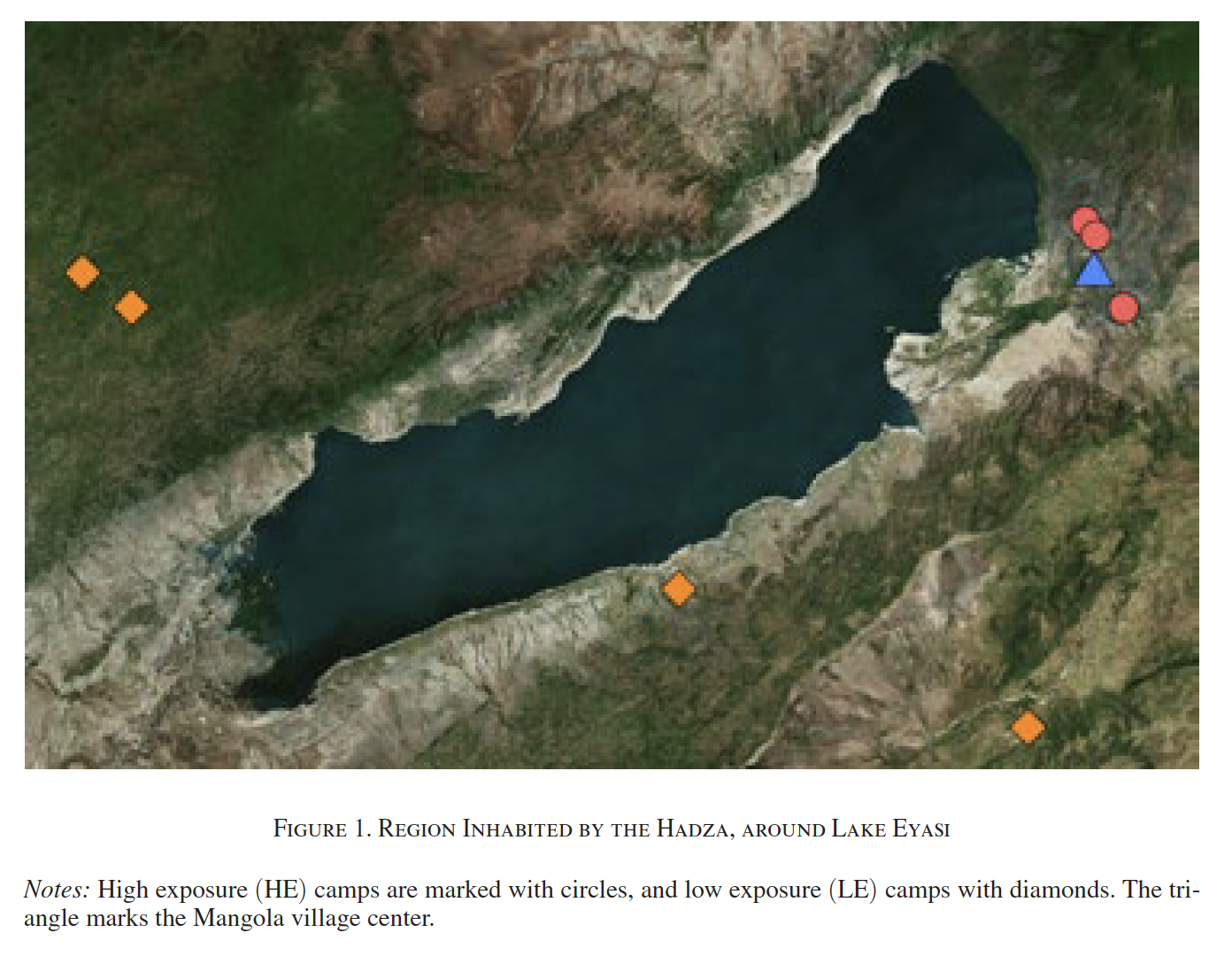
Reproduced from Apicella et al. (2014)
Hadze are genetically and culturally identical to their counterparts far from Mangola. So if we see WTA > WTP only in camps close to the village, then it can plausibly be explained by exposure to markets, suggesting that loss aversion is a learned trait. That is exactly what the authors find.
To estimate the treatment effect the authors run a simple linear probability model on whether a tribesperson traded their endowed good (tribespeople with loss aversion should be less likely to trade):
\[\text{trade} = \alpha + \beta\text{Magnola} + \gamma\mathbf{X} + \epsilon\]where Magnola is the treatment indicator (a tribesperson is in a camp near Mangola) and $\mathbf{X}$ is a set of controls.
Estimating $\mathbb{E}[\beta]$, the treatment effect, is straightforward. But what about $\mathbb{V}[\beta]$? The argument is that the standard errors should be clustered at the camp level. If there is “something in the water” (e.g., some tribespeople sharing observations about the experiment with each other), it must be accounted for when estimating the variance of the treatment effect.
Let’s replicate the paper’s headline result (Table 1 Column 5) by hand, coefficients and clustered standard errors.
1
2
# I downloaded the data from the AEA website
endowment_df = read_csv("apicella_al_2011.csv")
First we need to estimate the coefficients. Let’s create a model matrix from the data:
1
2
3
4
5
6
7
8
9
10
11
X = endowment_df %>%
  # create the interaction effect
  mutate(lighter_times_distance = lighter * distance_to_mangola) %>%
  # select the variables we want
  select(magnola_region, distance_to_mangola, lighter, lighter_times_distance) %>%
  # create an intercept
  mutate(intercept = 1) %>%
  # move the intercept to the front (not necessary but makes output match summary())
  relocate(intercept) %>%
  # convert to a matrix
  as.matrix()
and the response variable:
1
2
# same as `y = endowment_df$trade`
y = endowment_df %>% pull(trade)
and $n$ and $k$:
1
2
3
4
# number of observations
n = nrow(X)
# number of variables in the model (including the intercept)
k = ncol(X)
Our coefficients are estimated by $(X’ X)^{-1} X’y$ (note: crossprod(X) calculates $X’ X$ and %*% is element-wise matrix multiplication):
1
betas = solve(crossprod(X)) %*% crossprod(X,y)
Next we need the residuals, the estimates of the errors, which are just the observed outcomes (y) minus the predicted outcomes, $X\hat{\beta}$:
1
2
3
4
# predicted outcomes
y_pred = X %*% betas
# residuals
u = y - y_pred
OK, if we didn’t cluster the standard errors, and didn’t account for heteroskedasticity, we could just calculate them as
\[\mathbb{V}[\beta] = \frac{\hat{\epsilon}' \hat{\epsilon}}{n - k} (X'X)^{-1}\]1
vcov_nonclustered = sum(u^2)/(n - k) * solve(crossprod(X))
then take the square root of the diagonal of the matrix:
1
se_nonclustered = sqrt(diag(vcov_nonclustered))
and when we print the results:
1
cbind(betas, se_nonclustered)
1
2
3
4
5
6
                                    se_nonclustered
intercept               0.496564572     0.153222199
magnola_region         -0.285900185     0.145627602
distance_to_mangola     0.001436815     0.002626839
lighter                 0.079017343     0.098073004
lighter_times_distance -0.002968781     0.002271535
and you see we get the same results from feols (or lm):
1
2
endowment_model = fixest::feols(trade ~ magnola_region + distance_to_mangola + lighter + lighter*distance_to_mangola, data= endowment_df)
summary(endowment_model)
1
2
3
4
5
6
7
8
9
10
11
12
OLS estimation, Dep. Var.: trade
Observations: 182
Standard-errors: IID
                             Estimate Std. Error   t value Pr(>|t|)
(Intercept)                  0.496565   0.153222  3.240814 0.001424 **
magnola_region              -0.285900   0.145628 -1.963228 0.051186 .
distance_to_mangola          0.001437   0.002627  0.546975 0.585085
lighter                      0.079017   0.098073  0.805699 0.421497
distance_to_mangola:lighter -0.002969   0.002272 -1.306950 0.192925
---
Signif. codes:  0 '***' 0.001 '**' 0.01 '*' 0.05 '.' 0.1 ' ' 1
RMSE: 0.464483   Adj. R2: 0.07273
Clustering, finally
Now let’s cluster the standard errors.
First we need to calculate the variance-covariance matrix for each village or camp.
What camps are there?
1
2
3
camps = unique(endowment_df$campname)
n_camps = length(camps)
print(camps)
1
2
[1] "Endadubu"     "Mayai"        "Mwashilatu"   "Setako Chini" "Mizeu"        "Mkwajuni"     "Sonai"
[8] "Shibibunga"
So we have 8 variance-covariance matrices in $\Omega$. The plan is:
- Create an empty list of length 8
- Calculate each variance-covariance matrix and add it to the list
- Then add up all the matrices in the list to get $\Omega$.
Step 1:
1
2
3
4
5
6
# create the empty list
list_of_vcovs = vector(mode = "list", length = n_camps)
# name each element by camp
names(list_of_vcovs) = camps
# view it
list_of_vcovs
Step 2 requires us to loop over the data, grab the observations for each cluster and the residuals for each cluster, do the calculation, then add the resulting matrix to the list:
1
2
3
4
5
6
7
8
9
10
11
12
13
for(camp in camps) {
  # c is a vector of True/False
  ## it tells us the *indices* where an observation belongs to camp or not
  c = endowment_df$campname == camp
  # now we can subset our data by those indices..
  X_c = X[c, , drop = FALSE]
  #...and the residuals
  u_c = u[c]
  # then do the calculation u_c u_c'
  vcov_c = t(X_c) %*% tcrossprod(u_c) %*% X_c
  # add this matrix to the list
  list_of_vcovs[[camp]] = vcov_c
}
Now we need to reduce these 8 matrices into one matrix by adding them up element-wise (i.e., add the $i,j$ element of each matrix together). We can do this with Reduce():
1
2
# Reduce() cannot take named lists, so we need to unname() first
omega = Reduce(f = "+", x = unname(list_of_vcovs))
and now we can calculate the variance-covariance matrix and the standard errors:
1
2
3
4
5
6
# variance-covariance matrix
vcov = (solve(crossprod(X)) %*% omega %*% solve(crossprod(X))) * n_camps/(n_camps-1) * (n-1)/(n-k)
# standard errors
se_clustered = sqrt(diag(vcov))
# print the coefficients and standard errors
cbind(betas, se_clustered)
1
2
3
4
5
6
                                    se_clustered
intercept               0.496564572  0.095157351
magnola_region         -0.285900185  0.082226213
distance_to_mangola     0.001436815  0.001552297
lighter                 0.079017343  0.085915473
lighter_times_distance -0.002968781  0.001621867
and look how they line up nicely with the canned procedure from fixest:
1
2
# for more on clustering with fixest see https://lrberge.github.io/fixest/articles/standard_errors.html
summary(endowment_model, cluster = "campname")
1
2
3
4
5
6
7
8
9
10
11
12
OLS estimation, Dep. Var.: trade
Observations: 182
Standard-errors: Clustered (campname)
                             Estimate Std. Error   t value Pr(>|t|)
(Intercept)                  0.496565   0.095157  5.218352 0.001228 **
magnola_region              -0.285900   0.082226 -3.476996 0.010308 *
distance_to_mangola          0.001437   0.001552  0.925606 0.385450
lighter                      0.079017   0.085915  0.919710 0.388318
distance_to_mangola:lighter -0.002969   0.001622 -1.830471 0.109869
---
Signif. codes:  0 '***' 0.001 '**' 0.01 '*' 0.05 '.' 0.1 ' ' 1
RMSE: 0.464483   Adj. R2: 0.07273
Appendix
This exercise introduced me to the base::Reduce() function. It’s pretty cool. We used it above to do component-wise addition across matrices – adding $i$ and $j$ of each matrix together.
Check out this simpler example. Here is a list of two random $2 \times 2$ matrices:
1
2
3
mats = list(matrix(data = sample.int(20), 2, 2),
            matrix(data = sample.int(20), 2, 2))
print(mats)
1
2
3
4
5
6
7
8
9
[[1]]
     [,1] [,2]
[1,]   16   12
[2,]    5   15

[[2]]
     [,1] [,2]
[1,]    3    5
[2,]    4    2
We can do component-wise addition using a nested loop:
1
2
3
4
5
6
7
reduce_mats = matrix(data = NA, nrow = 2, ncol = 2)
for(i in 1:nrow(m)){
  for(j in 1:ncol(m)){
    reduce_mats[i,j] = mats[[1]][i,j] + mats[[2]][i,j]
  }
}
print(reduce_mats)
1
2
3
     [,1] [,2]
[1,]   19   17
[2,]    9   17
or more simply with Reduce():
1
Reduce(x = mats, f = "+")
1
2
3
     [,1] [,2]
[1,]   19   17
[2,]    9   17
Code
The code to reproduce the figures is on GitHub.